
East Tennessee State University East Tennessee State University
Digital Commons @ East Digital Commons @ East
Tennessee State University Tennessee State University
Electronic Theses and Dissertations Student Works
5-2017
A Distribution of the First Order Statistic When the Sample Size is A Distribution of the First Order Statistic When the Sample Size is
Random Random
Vincent Z. Forgo Mr
East Tennessee State University
Follow this and additional works at: https://dc.etsu.edu/etd
Part of the Statistical Theory Commons
Recommended Citation Recommended Citation
Forgo, Vincent Z. Mr, "A Distribution of the First Order Statistic When the Sample Size is Random" (2017).
Electronic Theses and Dissertations.
Paper 3181. https://dc.etsu.edu/etd/3181
This Thesis - unrestricted is brought to you for free and open access by the Student Works at Digital Commons @
East Tennessee State University. It has been accepted for inclusion in Electronic Theses and Dissertations by an
authorized administrator of Digital Commons @ East Tennessee State University. For more information, please
contact [email protected].

A Distribution of the First Order Statistic when the Sample Size is Random
A thesis
presented to
the faculty of the Department of Mathematics
East Tennessee State University
In partial fulfillment
of the requirements for the degree
Master of Science in Mathematical Sciences
by
Vincent Forgo
May 2017
Bob Price, Ph.D., Chair
Nicole Lewis, Ph.D.
JeanMarie Hendrickson, Ph.D.
Keywords: First order statistic, random sample size, Cumulative density function,
Probability density function, Expectation, Variance, Percentile
ABSTRACT
A Distribution of the First Order Statistic when the Sample Size is Random
by
Vincent Forgo
Statistical distributions also known as probability distributions are used to model
a random experiment. Probability distributions consist of probability density func-
tions (pdf) and cumulative density functions (cdf). Probability distributions are
widely used in the area of engineering, actuarial science, computer science, biological
science, physics, and other applicable areas of study. Statistics are used to draw con-
clusions about the population through probability models. Sample statistics such as
the minimum, first quartile, median, third quartile, and maximum, referred to as the
five-number summary, are examples of order statistics. The minimum and maximum
observations are important in extreme value theory. This paper will focus on the
probability distribution of the minimum observation, also known as the first order
statistic, when the sample size is random.
2
ACKNOWLEDGMENTS
I am grateful for the great support from the faculty of Department of Mathematics
and Statistics at East Tennessee State University. I appreciate the tremendous work
by committee members: Dr. Robert Price (committee and department Chair), Dr.
Nicole Lewis, and Dr. JeanMarie Hendrickson for making this paper possible. I am
more grateful to Dr. Robert Price for how instrumental He has being throughout this
paper.
3
TABLE OF CONTENTS
ABSTRACT . . . . . . . . . . . . . . . . . . . . . . . . . . . . . . . . . . 2
ACKNOWLEDGEMENTS . . . . . . . . . . . . . . . . . . . . . . . . . . 3
1 INTRODUCTION . . . . . . . . . . . . . . . . . . . . . . . . . . . . 5
2 FIXED SAMPLE SIZE . . . . . . . . . . . . . . . . . . . . . . . . . . 7
3 TRUNCATED POISSON MIXTURE . . . . . . . . . . . . . . . . . . 9
3.1 Uniform - Truncated Poisson Mixture Distribution . . . . . . 10
3.2 Exponential - Truncated Poisson Mixture Distribution . . . . 16
4 TRUNCATED BINOMIAL MIXTURE . . . . . . . . . . . . . . . . . 18
4.1 Uniform-Truncated Binomial Mixture Distribution . . . . . . . 19
4.2 Exponential-Truncated Binomial Mixture Distribution . . . . 22
5 TRUNCATED GEOMETRIC MIXTURE . . . . . . . . . . . . . . . 24
5.1 Uniform-Truncated Geometric Mixture . . . . . . . . . . . . . 25
5.2 Exponential-Truncated Geometric Mixture . . . . . . . . . . . 28
6 CONCLUSION . . . . . . . . . . . . . . . . . . . . . . . . . . . . . . 30
REFERENCES . . . . . . . . . . . . . . . . . . . . . . . . . . . . . . . . . 31
VITA . . . . . . . . . . . . . . . . . . . . . . . . . . . . . . . . . . . . . . 32
4
1 INTRODUCTION
The concept of order statistics is familiar in areas of finance and insurance (Risk
assessment). The order statistics of a random sample X
1
, X
2
, ...X
n
are defined as
X
(1)
≤ X
(2)
≤ .... ≤ X
(n)
. A situation can occur in actuarial science with a joint
life insurance. The policy pays out when one of the spouse’s dies. In this problem,
we want to know the distribution of the minimum payment, which is the random
variable of the two life spans. Another form of application of order statistics is about
a machine, which may run on 15 batteries and shuts off when the seventh battery
dies. We may want to know the distribution of X
(7)
. Thus, the distribution of the
random variable of the seventh longest lasting battery.
In order statistics the variables are considered as independent and identically
distributed, iid. The cumulative distribution function of the n
th
order statistic is
given as
F
n
(x) = P {allX
i
≤ x} = [P (X ≤ x)]
n
= [F
n
(x)]
n
.
This implies the cumulative distribution is F
n
(x) for this random variable. The
cumulative distribution function (cdf) of the first order statistic or the minimum is
(1 − P [(X
i
> x)])
n
.
The general formula of the cumulative distribution for the k
(th)
order statistic is given
as
n
X
j=k
n
j
F (x)
j
(1 − F (x))
n−j
.
5
Order statistics is among the most essential functions of a set of random variables that
are studied in probability and statistics. There is natural interest in studying the highs
and lows of a sequence, and the order statistics help in understanding concentration of
probability in a distribution[4]. It is important to note that the variables in the sample
are independent and identically distributed but because of the the sequential order
associated with order statistics, the order statistics is not distributed identically and
independently. Since the variables in the sample appear in order, there is a minimum
and maximum order statistics. Therefore, the n
th
(maximum) order statistic has a
pdf of
f
x(n)
= n[F (x)]
n−1
f(x)
and the first order statistic(minimum) will have a pdf of
f
x(1)
= n[1 − F (x)]
n−1
.
6
2 FIXED SAMPLE SIZE
Now let us consider X
i
to be iid continuous random variables i.e. all the random
variables have equal probability distribution and mutually independent of each other
such that the random variables follow a uniform distribution, X
i
∼ unif(0, 1) and
Z = min(X
1
, ...., X
n
). If n is fixed then
P (Z ≤ z) = 1 − P (Z > z) = 1 − [1 − F
X
(z)]
n
= 1 − [1 − z]
n
, 0 ≤ z ≤ 1.
where F
x
(z) is the cdf of the uniform distribution. The idea, of starting with 1 −
P (Z > z) is because we can say that if the first order statistics is the smallest,
then automatically z is less than Z. Hence we can find P (Z ≤ z) by starting with
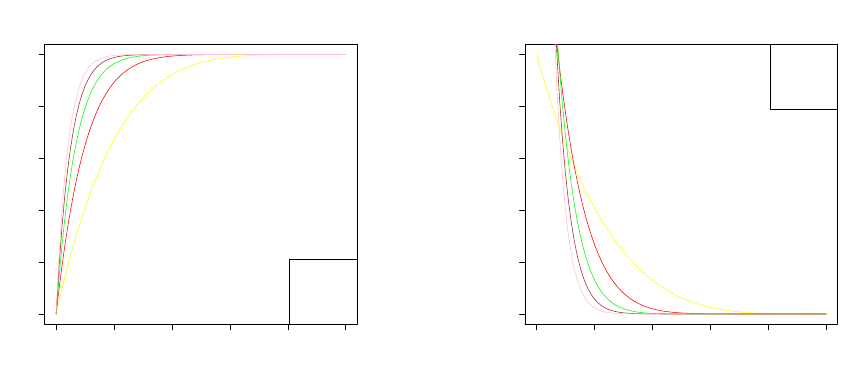
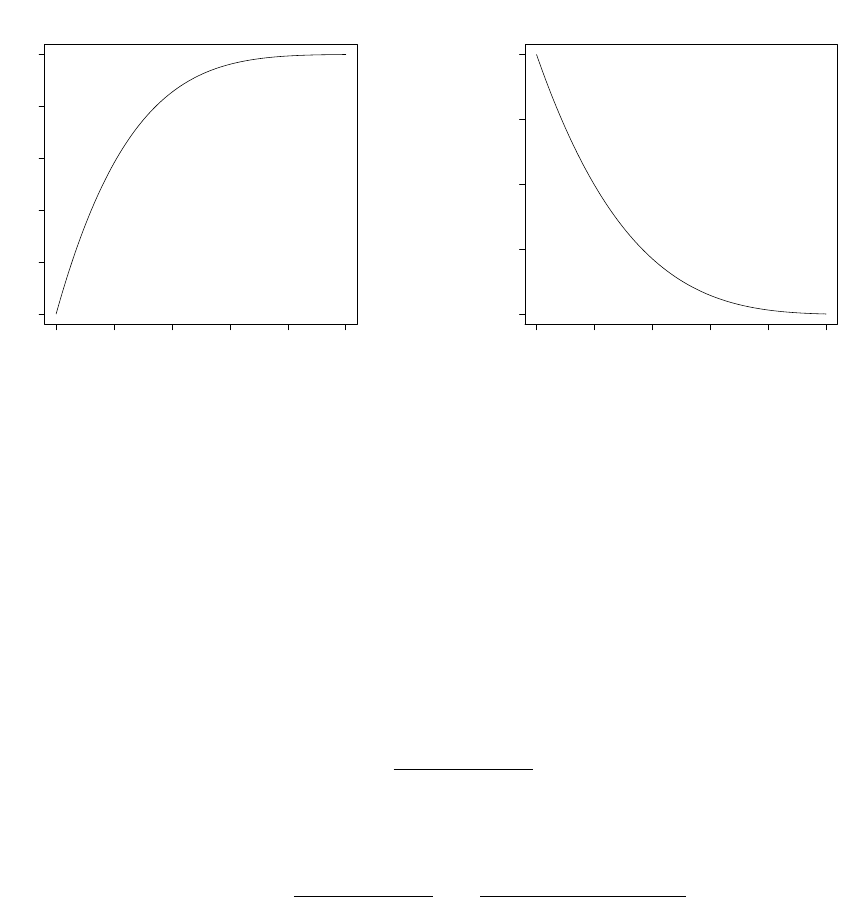
1 − P (Z > z). The pdf is generated by taking the derivative of the cdf which gives
f(z) = n[1 − z]
n−1
. The cdf and pdf is graphically shown in figure 1 and becomes
steeper as n gets large.
7
0.0 0.2 0.4 0.6 0.8 1.0
0.0 0.2 0.4 0.6 0.8 1.0
x
f(x)
n=5,yellow
n=10,red
n=15,green
n=20,brown
n=25,pink
(a) Cummulative distribution function plots for
different sample sizes.
0.0 0.2 0.4 0.6 0.8 1.0
0 1 2 3 4 5
x
f(x)
n=5,yellow
n=10,red
n=15,green
n=20,brown
n=25,pink
(b) Probability density function plots for different
sample sizes.
Figure 1: The cdf and pdf of the smallest order statistic when the underlying distri-
bution is uniform.
8

3 TRUNCATED POISSON MIXTURE
The Poisson distribution is a discrete probability distribution. The Poisson distri-
bution is some times truncated, i.e. the random variables are assigned numbers that
are greater than zero. The Poisson distribution is a discrete distribution used for the
interval counts of events that randomly occur in given interval (or space)[3]. The
probability mass function (pmf) is
P (N = n) =
λ
n
e
−λ
n!
, n = 0, 1, 2, 3...; λ > 0.
with expectation E(N) = λ and variance V (N) = λ. The probability generating
function of the Poisson distribution is G(t) = e
λ(t−1)
and the moomemt generating
function (mgf) is M(t) = e
λ(e
t
−1)
, where the events occur on a given time t.
The truncated Poisson is a discrete probability distribution which is used to de-
scribe events that occur per unit time and can not be a zero event. In this case,
the starting point will not be zero but 1. This process is termed as the truncated
Poisson distribution or the zero truncated Poisson distribution. The pmf of the zero
truncated Poisson is given below as
P (N = n) =
λ
n
e
−λ
(1 − e
−λ
)n!
, n = 1, 2 . . . .
with an expectation of E(N ) =
λ
1−e
−λ
and a variance of V (N) =
λ
(1−e
−λ
)
2
.
If the random variable X
i
follows a continuous probability distribution and Z|N =
min(X
1
, ...., X
n
), then we can find a distribution for the first other statistic X
(1)
when
the sample size is fixed or random. In the next section, the paper will focus more on a
general formula for finding the cdf and pdf of a random variable with any continuous
probability distribution like uniform, exponential, etc. and a random sample size(N).
9

If N is a random sample size and follows a truncated Poisson distribution then
for any continuous distribution of X
i
, we can find the cdf of the distribution by using
the generalised formula for P (Z > z), i.e,
P (Z > z) =
X
n
[1 − F
x
(z)]
n
e
−λ
λ
n
(1 − e
−λ
)n!
=
e
−λ
(1 − e
−λ
)
[e
(1−F
x
(z))λ
− 1].
The general cdf will be
F (z) = 1 −
e
−λ
(1 − e
−λ
)
[e
(1−F
x
(z))λ
− 1]
with a pdf
f(z) =
λe
−λ
1 − e
−λ
f
x
(z)[e
(1−F
x
(z)λ
], λ > 0,
where F
x
(z) and f
x
(z) are the cdf and pdf of the continuous random variable X
i
,
respectively. If X
i
follows a continuous distribution which is not closed like the
normal distribution, then we can use R functions like the pnorm and dnorm to find
the cdf and pdf respectively, i.e., F
x
(z) = pnorm(x) and f
x
(z) = dnorm(x).
3.1 Uniform - Truncated Poisson Mixture Distribution
If the random variable X
i
follows a continuous probability distribution and Z =
min(X
1
, ...., X
N
) , then we can find a distribution for the first other statistic X
(1)
.
In this section we are focused on a distribution of the first order statistics with
an underlying uniform distribution and a random sample which follows a truncated
Poisson distribution. If N is random then
P (Z > z) =
X
n
P (Z > z|N = n)P (N = n), 0 < z < 1
10

where P (Z > z|N ) is the conditional distribution and P (N = n) is the marginal
distribution. The idea of N being random will be widely explored in this paper. Our
new distribution is mainly based on the idea of first order statistics and N following
truncated Poisson. Let us consider X
i
∼ Unif(0, 1) and Z|N = min {X
1
, X
2
, ...., X
N
}
where N is sample size and is random with distribution
P (N = n) =
e
−λ
λ
n
(1 − e
−λ
)n!
, n = 1, 2, 3, . . . .
Then
P (Z > z) =
∞
X
n=1
(1 − z)
n
e
−λ
λ
n
(1 − e
−λ
)n!
=
∞
X
n=0
(1 − z)
n
e
−λ
λ
n
(1 − e
−λ
)n!
− (1 − z)
0
e
−λ
λ
0
(1 − e
−λ)
0!
=
e
−λ
(1 − e
−λ
)
P
∞
n=0
((1 − z)λ)
n
n!
−
e
−λ
(1 − e
−λ
)
.
Using the definition of
P
∞
n=0
λ
n
n!
= e
λ
we can simplify the above equation as
e
−λ
(1 − e
−λ
)
[e
(1−z)λ
− 1].
Hence the cumulative distribution function (cdf) is given as F (z) = 1−
e
−λ
(1−e
−λ
)
[e
(1−z)λ
− 1].
where 0 < z < 1, λ > 0.
The probability density function (pdf) can be derived by taking the derivative of
the cdf with respect to z. The pdf of a first order statistic when the underlying
distribution is uniform with a random sample that is a truncated Poisson is
f(z) =
λe
−λ
1 − e
−λ
[e
(1−z)λ
], 0 < z < 1, λ > 0.
11

It can be proven that f(z) satisfies the conditions of a pdf i.e.
R
1
0
f(z)dz = 1
Z
1
0
f(z)dz =
Z
1
0
λe
−λ
1 − e
−λ
[e
(1−z)λ
]dz =
λe
−λ
1 − e
−λ
Z
1
0
[e
(1−z)λ
]
1
e
λ
− 1
[e
λ
− 1] = 1.
From the distribution generated, the expectation is given as
E(Z) =
Z
1
0
λe
−λ
1 − e
−λ
z[e
(1−z)λ
]dz =
e
λ
− λ − 1
λ(e
λ
− 1)
.
The moment generating function (mgf) can be used to estimate both the
expectation and variance. The mgf of the distribution is given as
M(t) = E(e
tz
) =
Z
1
0
e
tz
f(z)dz =
Z
1
0
e
tz
e
−λ
1 − e
−λ
e
(1−z)λ
dz
=
λe
−λ
1 − e
−λ
e
λ
− e
t
λ − t
.
12
0.0 0.2 0.4 0.6 0.8 1.0
0.0 0.2 0.4 0.6 0.8 1.0
x
f(x)
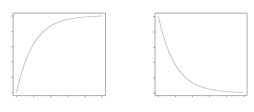
(a) Cumulative distribution function plot
0.0 0.2 0.4 0.6 0.8 1.0
0 1 2 3 4 5
x
f(x)
(b) Probability density function plot
Figure 2: The cdf and pdf of the smallest order statistic when the underlying distri-
bution is uniform and random sample size which follows a truncated Poisson where
rate (λ) = 5.
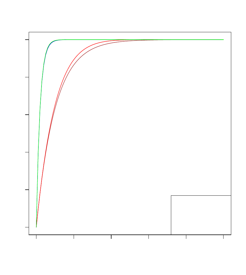
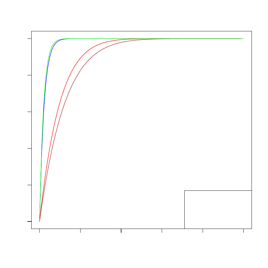
From Figure 3, it is clear that the cdf in both the random and fixed cases tend to be
the same as λ and n increases. The behaviour of the cdf as λ and n increases shows
a steep and sharp turn closer to 1. This implies that the larger n and λ gets, the
more steeper the curve becomes and the fixed sample size (n) and the random
sample size (N) all tend to have the same cdf.
13
0.0 0.2 0.4 0.6 0.8 1.0
0.0 0.2 0.4 0.6 0.8 1.0
x
f(x)
lambda=10,brown
n=10,red
lambda=50,blue
n=50,green
Figure 3: A cumulative distribution function plots of different samples (n) and differ-
ent rates (λ) when the underlying distribution is uniform for fixed sample and random
sample which follows a truncated Poisson.
14

The percentile function is relevant in statistics because it can be used to indicate
the value below a certain percentage. The percentile function can also be used to
calculate the lower quartile(Q
1
), median(Q
2
) and the upper quartile(Q
3
). The
percentile function of the first order statistic when the underlying distribution is
uniform and a random sample size that follows a truncated Poisson is
P = F (µ) =
Z
µ
−∞
f(y)dy.
where f(y) is the probability density function(pdf). From the uniform truncated
Poisson distribution, the probability distribution function pdf is
λe
−λ
1−e
−λ
[e
(1−z)λ
− 1], λ > 0. The percentile function is generated by
Z
µ
0
λe
−λ
1 − e
−λ
[e
(1−z)λ
]dz =
λe
−λ
1 − e
−λ
Z
µ
0
[e
(1−z)λ
]dz
=
e
−λ
1 − e
−λ
(e
λ
− e
λ(1−µ)
)
P =
e
−λ
1 − e
−λ
(e
λ
− e
λ(1−µ)
), λ > 0, µ > 0
From the above percentile equation, the 50th percentile(median) is calculated in terms
of λ as
0.5 =
e
λ
− e
λ(1−µ)
e
λ
− 1
⇒ µ =
λ − log(1 − e
λ
)
0.5 +
e
λ
1−e
λ
λ
.
15

3.2 Exponential - Truncated Poisson Mixture Distribution
In this section, we are focused on a distribution of the first order statistics with an
underlying exponential distribution and a random sample which follows a truncated
Poisson. If Z|N = min {X
1
, ...., X
N
}, where N is the sample size which is random
with a distribution
P (N = n) =
e
−λ
λ
n
(1 − e
−λ
)n!
.
We have
P (Z > z) =
∞
X
n=1
(e
−zµ
)
n
e
−λ
λ
n
(1 − e
−λ
)n!
P (Z > z) =
∞
X
n=1
e
−λ−znµ
λ
n
(1 − e
−λ
)n!
=
∞
X
n=0
e
−λ−znµ
λ
n
(1 − e
−λ
)n!
−
e
−λ
1 − e
−λ
=
e
−λ
1 − e
−λ
∞
X
n=0
e
−znµ
λ
n
n!
− 1
=
e
−λ
(1 − e
−λ
)
[e
λe
−zµ
− 1].
The cdf of an underlying exponential distribution with a random sample size which
follows a truncated Poisson is
F (z) = 1 −
e
−λ
1 − e
−λ
[e
λe
−zµ
− 1], λ > 0, z > 0, µ > 0.
and a pdf of
f(z) =
d
dz
1 −
e
−λ
1 − e
−λ
[e
λe
−zµ
− 1]
=
λµ
e
λ
− 1
[e
λe
−zµ
−zµ
], λ > 0, z > 0, µ > 0.
16
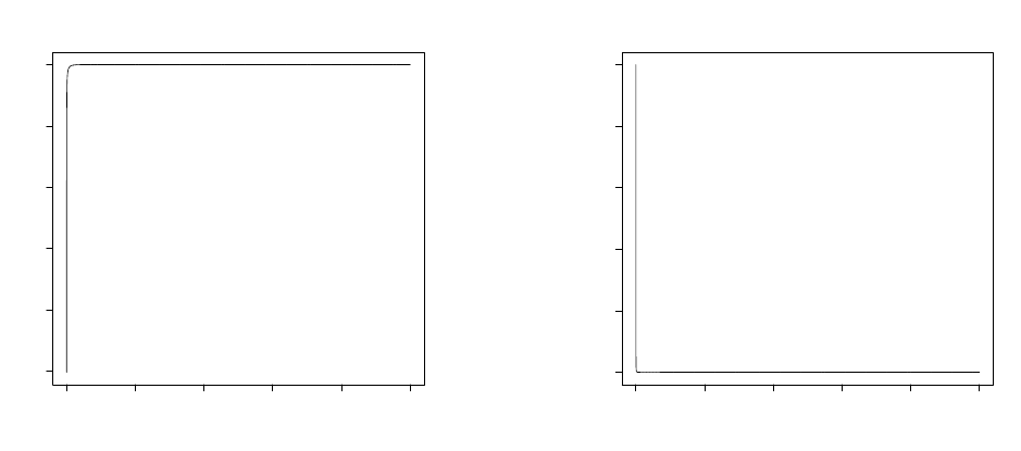
0 2000 4000 6000 8000 10000
0.0 0.2 0.4 0.6 0.8 1.0
Index
F0
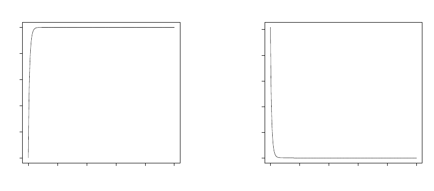
(a) Cumulative density function plot.
0 2000 4000 6000 8000 10000
0.0 0.5 1.0 1.5 2.0 2.5
Index
F0
(b) Probability density function plot.
Figure 4: A figure representing the cdf and pdf with an underlying exponential dis-
tribution and a random sample size which follows a truncated Poisson when rate
(λ) = 0.5 and µ = 1.
17

4 TRUNCATED BINOMIAL MIXTURE
The truncated binomial distribution is a discrete probability distribution with a
probability mass function
P (N = n) =
k
n
p
n
(1 − p)
k−n
1 − (1 − p)
k
for n = 1, 2, ...k. Where k is the number of success and p is the probability of success
with an expectation
E(N) =
kp
1 − (1 − p)
k
and a variance
V (N) =
kp(1 − p − (1 − p + kp))(1 − p)
k
(1 − (1 − p)
k
)
2
.
The binomial distribution is often used to model the number of success(k) among a
sample of size(n).
In this section of the paper, we will focus on finding a general cdf and pdf when
the random sample size follows a truncated binomial distribution and the random
variable X
i
follows a continuous distribution that can be exponential, uniform, etc.
The general formula for P (Z > z) will be
P (Z > z) =
P
n
[1 − F
x
(z)]
n
k
n
p
n
(1 − p)
k−n
1 − (1 − p)
k
=
1
1 − (1 − p)
k
(1−F
x
(z)p)
k
−(1−p)
k
.
The general cdf will be
F (z) = 1 −
1
1 − (1 − p)
k
(1 − F
x
(z)p)
k
− (1 − p)
k
18

and a pdf of
f(z) =
kp(1 − F
x
(z)p)
k−1
f
x
(z)
1 − (1 − p)
k
, 0 ≤ p ≤ 1,
where F
x
(z) and f
x
(z) are the cdf and pdf of the continuous random variable X
i
respectively.
4.1 Uniform-Truncated Binomial Mixture Distribution
In this section, we are focused on finding a distribution of the first order statistics
with an underlying uniform distribution and a random sample which follows a trun-
cated binomial distribution. If Z|N = min {X
1
, ...., X
N
} where N is the sample size
which is random with a distribution
P (N = n) =
k
n
p
n
(1 − p)
k−n
1 − (1 − p)
k
for n=1, 2, ...k. This implies that
P (Z>z)=
P
k
n=1
(1 − z)
n
k
n
p
n
(1 − p)
k−n
1 − (1 − p)
k
=
1
1 − (1 − p)
k
k
X
n=1
(1 − z)
n
k
n
p
n
(1 − p)
k−n
=
1
1 − (1 − p)
k
k
X
n=0
(1 − z)
n
k
n
p
n
(1 − p)
k−n
− (1 − p)
k
=
1
1 − (1 − p)
k
k
X
n=0
k
n
((1 − z)p)
n
(1 − p)
k−n
− (1 − p)
k
=
1
1 − (1 − p)
k
((1 − z)p + (1 − p))
k
− (1 − p)
k
=
1
1 − (1 − p)
k
(1 − zp)
k
− (1 − p)
k
.
Thus the cdf of an underlying uniform distribution with a random sample which
follows a truncated binomial distribution is
F (z)=1 −
1
1 − (1 − p)
k
(1 − zp)
k
− (1 − p)
k
19
0.0 0.2 0.4 0.6 0.8 1.0
0.0 0.2 0.4 0.6 0.8 1.0
x
f(x)
(a) Cumulative distribution function plot with k=
5 and p=0.8.
0.0 0.2 0.4 0.6 0.8 1.0
0 1 2 3 4
x
f(x)
(b) Probability density function plot with k=5 and
p=0.8.
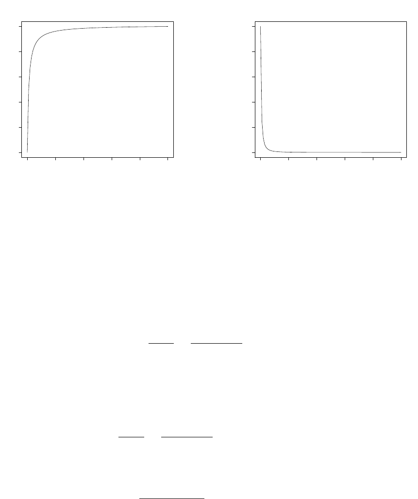
Figure 5: A figure representing the cdf and pdf with an underlying uniform distribu-
tion and random sample size which follows truncated binomial.
with a probability density function
f(z)=
kp(1 − zp)
k−1
1 − (1 − p)
k
and
E(Z)=
Z
1
0
z
kp(1 − zp)
k−1
1 − (1 − p)
k
dz=
1 − (1 − p)
k
(kp + 1)
p(k + 1)
.
Figure 5a shows the cdf of an underlying uniform distribution and a random
sample size that follows truncated binomial distribution. Figure 5b is the pdf of an
underlying uniform distribution and a random sample size which follows a truncated
binomial distribution.
20
0.0 0.2 0.4 0.6 0.8 1.0
0.0 0.2 0.4 0.6 0.8 1.0
x
f(x)
K=10,P=0.8,brown
n=10,red
k=50,p=0.9,blue
n=50,green
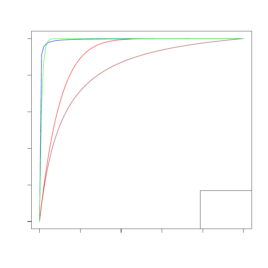
Figure 6: A cumulative distribution function plots of different samples (n) and differ-
ent p and k when the underlying distribution is uniform for fixed sample and random
sample that follows a truncated binomial.
From Figure 6, it is clear that the cdf in both the random and fixed cases tend to
be the same as p, k and n increases. The behaviour of the cdf as p, k and n increases
21

shows a steep and sharp turn closer to 1. This implies that the larger p, k and n gets,
the steeper the curve becomes.
The percentile function of an underlying uniform distribution with a random sam-
ple size which follows a truncated binomial distribution is given as
P =
Z
µ
0
kp(1 − zp)
k−1
1 − (1 − p)
k
dz=
(1 − µp)
k
− 1
(1 − p)
k
− 1
.
From the Percentile function, the 50th percentile (µ) or the median is calculated using
the relation
P =
(1 − pµ)
k
− 1
(1 − p)
k
− 1
Hence
µ=
1 − (0.5 −
1
1−(1−p)
k
)((1 − p)
k
− 1))
p
0≤p≤1, P =0.5 and 0<z<1.
4.2 Exponential-Truncated Binomial Mixture Distribution
In this section, we are focused on finding a distribution of the first order statistics
with an underlying exponential distribution and a random sample which follows a
truncated binomial distribution. If Z|N=min {X
1
, ...., X
N
} where N is the sample
size which is random with a distribution
P (N=n)=
k
n
p
n
(1 − p)
k−n
1 − (1 − p)
k
for n=1, 2, ...k . This implies that
P (Z>z)=
P
k
n=1
(e
−zµ
)
n
k
n
p
n
(1 − p)
k−n
1 − (1 − p)
k
=
1
1 − (1 − p)
k
k
X
n=1
(e
−zµ
)
n
k
n
p
n
(1 − p)
k−n
22

0 2000 4000 6000 8000 10000
0.0 0.2 0.4 0.6 0.8 1.0
Index
F0
(a) Cumulative distribution function plot when p=
0.2, k=5 and µ=1.
0 2000 4000 6000 8000 10000
0.0 0.5 1.0 1.5 2.0
Index
F0
(b) Probability density function plot when p=
0.8, k=5 and µ=1.
Figure 7: The cdf and pdf of the smallest order statistic when the underlying distri-
bution is exponential and random sample size which follows a truncated binomial.
1
1 − (1 − p)
k
k
X
n=0
(e
−zµ
)
n
k
n
p
n
(1 − p)
k−n
− (1 − p)
k
=
(pe
−zµ
+ 1 − p)
k
− (1 − p)
k
1 − (1 − p)
k
.
Thus the cdf of an underlying exponential distribution with a random sample which
follows a truncated binomial distribution is
F (z)=1 −
(pe
−zµ
+ 1 − p)
k
− (1 − p)
k
1 − (1 − p)
k
, µ>0, 0≤p≤1, z>0
with a probability density function
f(z)=kµp
1−k
e
−zµ
(pe
−zµ
− p + 1)
k−1
, µ>0, 0≤p≤1, z>0.
23

5 TRUNCATED GEOMETRIC MIXTURE
In this section of the paper, the focus will be finding a distribution of the first
order statistic when X
i
is any continuous distribution and the random sample size
follows a geometric distribution. The geometric distribution is a discrete probability
distribution which is used to represent the first outcome of a specific event with a
probability p of the event occurring. The pmf of the geometric distribution is
P (N=n)=p(1 − p)
n
, n=0, 1, 2, . . .
with an expectation
E(N)=
1 − p
p
and variance
V (N)=
1 − p
p
2
0≤p≤1.
The truncated geometric distribution is a modified form of the geometric distribution
with a probability mass function (pmf)
P (N=n)=p(1 − p)
n−1
, n=1, 2, . . .
with an expectation
E(N)=
1
p
and variance
V (N)=
1 − p
p
2
0≤p≤1.
24

If N follows a truncated geometric distribution then for any continuous distribution
of X
i
, the generalised formula for P (Z>z) will be
P (Z>z)=
X
n
P (Z>z|N =n)P (N=n)
=
∞
X
n=1
(1 − F
x
(z))
n
p(1 − p)
n−1
=p
∞
X
n=0
((1 − F
x
(z))(1 − p))
n
− (1 − p)
−1
.
The general cdf of an underlying continuous distribution with a random sample which
follows truncated geometric distribution is
F (z)=1 −
p
1 − p
−1
pF
x
(z) − p − F
x
(z)
− 1
and a pdf of
f(z)=
p
f
x
(z)(pF
x
(z) − p − F
x
(z))
2
0≤p≤1.
Where F
x
(z) and f
x
(z) are the cdf and pdf of the continuous random variable X
i
respectively.
5.1 Uniform-Truncated Geometric Mixture
The distribution of a first order statistic with an underlying uniform distribution if
Z|N=min {X
1
, ...., X
N
} where N is the random sample size which follows a truncated
geometric distribution
P (N=n)=p(1 − p)
n−1
, n=1, 2, . . . .
This implies
P (Z>z)=
∞
X
n=1
(1 − z))
n
p(1 − p)
n−1
=p
∞
X
n=0
((1 − z)(1 − p))
n
− (1 − p)
−1
25
0.0 0.2 0.4 0.6 0.8 1.0
0.0 0.2 0.4 0.6 0.8 1.0
x
f(x)
(a) Cumulative distribution function plot
0.0 0.2 0.4 0.6 0.8 1.0
0 20 40 60 80 100
x
f(x)
(b) Probability density function plot
Figure 8: A Figure representing the cdf and pdf with an underlying uniform distri-
bution and a random sample size which follows a truncated geometric distribution
when p=0.01.
=
p
1 − p
−1
zp − p − z
− 1
.
The cdf of a first order statistic with an underlying uniform distribution and a random
sample size which follows a truncated geometric distribution is
F (z)=1 −
p
1 − p
−1
zp − p − z
− 1
, 0≤p≤1, 0<z<1,
with a pdf of
f(z)=
p
(pz − p − z)
2
, 0≤p≤1, 0<z<1.
26
0.0 0.2 0.4 0.6 0.8 1.0
0.0 0.2 0.4 0.6 0.8 1.0
x
f(x)
P=0.1,brown
n=10,red
p=0.001,blue
n=100,green
Figure 9: A cumulative distribution function plots of different samples (n) and differ-
ent probabilities p when the underlying distribution is uniform for fixed and a random
sample which follows a truncated geometric .
From Figure 9, it is clear that the cdf in both the random and fixed cases tend to
take the similar shape as p decreases and n increases. The behaviour of the cdf as p
27

decreases and n increases shows a steep and sharp turn closer to 1. This implies that
the smaller p gets and the larger n gets, both fixed and random sample size tend to
have the same cdf.
5.2 Exponential-Truncated Geometric Mixture
The distribution of a first order statistic with an underlying exponential distribu-
tion if (Z|N )=min {X
1
, ...., X
N
} where N is the random sample size which follows a
truncated geometric distribution
P (N=n)=p(1 − p)
n−1
, n=1, 2, . . . .
P (Z>z)=
∞
X
n=1
(e
−zµ
))
n
p(1 − p)
n−1
=p
∞
X
n=0
((e
−zµ
(1 − p))
n
− (1 − p)
n−1
.
This implies
P (Z>z)=
pe
−zµ
(1 − (e
−zµ
))(1 − p)
.
Hence, the cdf of a first order statistic with an underlying exponential distribution
and a random sample size which follows a truncated geometric distribution is
F (z)=1 −
pe
−zµ
(1 − (e
−zµ
))(1 − p)
, rate(µ)>0, 0≤p≤1, z>0
with a pdf of
f(z)=
pµe
zµ
(e
zµ
+ p − 1)
2
, rate(µ)>0, 0≤p≤1, z>0.
28
0 2000 4000 6000 8000 10000
0.0 0.2 0.4 0.6 0.8 1.0
Index
f0
(a) Cumulative distribution function plot
0 2000 4000 6000 8000 10000
0 20 40 60 80 100
Index
F0
(b) Probability distribution function plot
Figure 10: The cdf and pdf of the smallest order statistic when the underlying dis-
tribution is exponential and random sample size which follows a truncated geometric
with p=0.01 and µ=1.
29
6 CONCLUSION
The paper has focused on finding probability distributions of the first-order statis-
tic when the sample size is random. The pivot of these joint distributions is a merge
between the marginal and conditional probability distribution. In some instances,
some properties that include the expectation, variance and percentile are calculated.
The primary objective of this paper is to consider a random sample size and compare
its behaviour to a fixed sample size in terms of their cumulative distribution func-
tions(cdf). A comparison between the cdf when the sample size is fixed and random
sample size is shown in figures 3, 6 and 9. It is clear at the end of the comparison
in figure 3 and 6 that, as the sample size(n) increases in the fixed case, the cdf ap-
proaches one and gets more steep. We see from figures 3 and 6 that as the sample
size increases and λ, p and k increases the cdf in both the fixed and random case
appear the same. In figure 9, as n increases and p decreases, both cdfs in the fixed
and random case take similar shape and becomes more steep and turns sharply close
to one.
30
REFERENCES
[1] Statistical inference 2nd Edition by George Cassela,Roger. L. Berger.
[2] Introduction to Mathematical Statistics, 7th edition, by Hogg, Robert V. Mckean,
and Allen T. Published by Pearson, 2013.
[3] The Poisson Distribution, by Jonathan Marchini, Nov 2008.
[4] Finite sample theory of order statistics and extremes, by Anirban DasGupta,
May 2011.
31
VITA
VINCENT FORGO
Education: B.S. Mathematics and Statistics, University of
Capecoast, Capecoast, Ghana 2009
M.S. Applied Mathematics, Indiana University of
Pennsylvania, Indiana, Pennsylvania 2014
M.S. Mathematical Science,
East Tennessee State University 2017
Professional Experience: Mathematics Teacher, S D A Senior High School,
Bekwai, Ghana, 2009–2011
Graduate Assistant, Indiana University of
Pennsylvania, Indiana, Pennsylvania, 2012–2013
Graduate Assistant, East Tennessee State
University, Johnson City, Tennessee, 2014–2016
Projects: Vincent Forgo, “A Distribution of the First
Order Statistic when the Sample Size is Random”
32
