Cumulative distribution

Title stata.com

cumul — Cumulative distribution

Description Quick start Menu Syntax

Options Remarks and examples Acknowledgment References

Also see

Description

cumul creates newvar, deﬁned as the empirical cumulative distribution function of varname.

Quick start

Create new variable ecd containing the empirical cumulative distribution of v

cumul v, gen(ecd)

Use frequency as the unit for v to generate ecdf

cumul v, gen(ecdf) freq

Give equal values of v the same value in generated ecde

cumul v, gen(ecde) equal

Graph the empirical cumulative distribution of v

line ecd v, sort

Graph the distributions of variables v1 and v2

cumul v1, gen(ecd1) equal

cumul v2, gen(ecd2) equal

stack ecd1 v1 ecd2 v2, into(ecd v) wide clear

line ecd1 ecd2 v, sort

Statistics > Summaries, tables, and tests > Distributional plots and tests > Generate cumulative distribution

2 cumul — Cumulative distribution

Syntax

cumul varname



 

weight



, generate(newvar)



options



options Description

Main

∗

generate(newvar) create variable newvar

freq use frequency units for cumulative

equal generate equal cumulatives for tied values

∗

generate(newvar) is required.

by is allowed; see [D] by.

fweights and aweights are allowed; see [U] 11.1.6 weight.

Options



 

Main



generate(newvar) is required. It speciﬁes the name of the new variable to be created.

freq speciﬁes that the cumulative be in frequency units; otherwise, it is normalized so that newvar

is 1 for the largest value of varname.

equal requests that observations with equal values in varname get the same cumulative value in

newvar.

Remarks and examples stata.com

Example 1

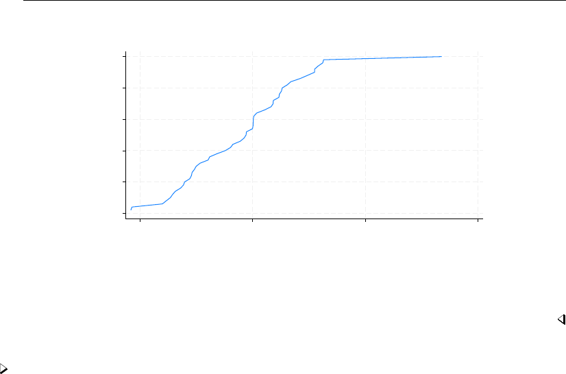
cumul is most often used with graph to graph the empirical cumulative distribution. For instance,

we have data on the median family income of 957 US cities:

. use https://www.stata-press.com/data/r18/hsng

(1980 Census housing data)

. cumul faminc, gen(cum)

. sort cum

. line cum faminc, ytitle("") xlabel(, format(%6.0f))

> title("Cumulative of median family income")

> subtitle("1980 Census, 957 US cities")

cumul — Cumulative distribution 3

15000 20000 25000 30000

Median family inc., 1979

1980 Census, 957 US cities

Cumulative of median family income

It would have been enough to type line cum faminc, but we wanted to make the graph look better;

see [G-2] graph twoway line.

If we had wanted a weighted cumulative, we would have typed cumul faminc [w=pop] at the

ﬁrst step.

Example 2

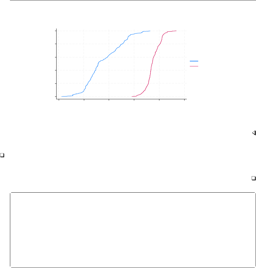
To graph two (or more) cumulatives on the same graph, use cumul and stack; see [D] stack. For

instance, we have data on the average January and July temperatures of 956 US cities:

. use https://www.stata-press.com/data/r18/citytemp, clear

(City temperature data)

. cumul tempjan, gen(cjan)

. cumul tempjuly, gen(cjuly)

. stack cjan tempjan cjuly tempjuly, into(c temp) wide clear

. line cjan cjuly temp, sort ytitle("") xtitle("Temperature (F)")

> title("Cumulatives:" "Average January and July temperatures")

> subtitle("956 US cities") legend(label(1 January) label(2 July))

4 cumul — Cumulative distribution

0 20 40 60 80 100

Temperature (F)

January

July

956 US cities

Cumulatives:

Average January and July temperatures

As before, it would have been enough to type line cjan cjuly temp, sort. See [D] stack for an

explanation of how the stack command works.

Technical note

According to Beniger and Robyn (1978), Fourier (1821) published the ﬁrst graph of a cumulative

frequency distribution, which was later given the name “ogive” by Galton (1875).

 

Jean Baptiste Joseph Fourier (1768–1830) was born in Auxerre in France. As a young man,

Fourier became entangled in the complications of the French Revolution. As a result, he was

arrested and put into prison, where he feared he might meet his end at the guillotine. When

he was not in prison, he was studying, researching, and teaching mathematics. Later, he served

Napolean’s army in Egypt as a scientiﬁc adviser. Upon his return to France in 1801, he was

appointed Prefect of the Department of Is

ere. While prefect, Fourier worked on the mathematical

basis of the theory of heat, which is based on what are now called Fourier series. This work

was published in 1822, despite the skepticism of Lagrange, Laplace, Legendre, and others—who

found the work lacking in generality and even rigor—and disagreements of both priority and

substance with Biot and Poisson.

 

Acknowledgment

The equal option was added by Nicholas J. Cox of the Department of Geography at Durham

University, UK, who is coeditor of the Stata Journal and author of Speaking Stata Graphics.

cumul — Cumulative distribution 5

References

Beniger, J. R., and D. L. Robyn. 1978. Quantitative graphics in statistics: A brief history. American Statistician 32:

1–11. https://doi.org/10.2307/2683467.

Fourier, J. B. J. 1821. Notions g

erales, sur la population. Recherches Statistiques sur la Ville de Paris et le

epartement de la Seine 1: 1–70.

Galton, F. 1875. Statistics by intercomparison, with remarks on the law of frequency of error. Philosophical Magazine

49: 33–46. https://doi.org/10.1080/14786447508641172.

Wilk, M. B., and R. Gnanadesikan. 1968. Probability plotting methods for the analysis of data. Biometrika 55: 1–17.

https://doi.org/10.2307/2334448.

Also see

[R] Diagnostic plots — Distributional diagnostic plots

[R] kdensity — Univariate kernel density estimation

[D] stack — Stack data

Stata, Stata Press, and Mata are registered trademarks of StataCorp LLC. Stata and

Stata Press are registered trademarks with the World Intellectual Property Organization

of the United Nations. StataNow and NetCourseNow are trademarks of StataCorp

LLC. Other brand and product names are registered trademarks or trademarks of their

respective companies. Copyright

 1985–2023 StataCorp LLC, College Station, TX,

For suggested citations, see the FAQ on citing Stata documentation.