STAT/Q SCI 403: Introduction to Resampling Methods Spring 2017
Lecture 1: CDF and EDF
Instructor: Yen-Chi Chen
1.1 CDF: Cumulative Distribution Function
For a random variable X, its CDF F(x) contains all the probability structures of X. Here are some properties
of F (x):
• (probability) 0 ≤ F (x) ≤ 1.
• (monotonicity) F (x) ≤ F(y) for every x ≤ y.
• (right-continuity) lim
x→y
+
F (x) = F (y), where y
+
= lim
>0,→0
y + .
• lim
x→−∞
F (x) = F (−∞) = 0.
• lim
x→+∞
F (x) = F (∞) = 1.
• P (X = x) = F (x) − F (x
−
), where x
−
= lim
<0,→0
x + .
Example. For a uniform random variable over [0, 1], its CDF
F (x) =
Z
x
0
1 du = x
when x ∈ [0, 1] and F (x) = 0 if x < 0 and F (x) = 1 if x > 1.
Example. For an exponential random variable with parameter λ, its CDF
F (x) =
Z
x
0
λe
−λu
du = 1 − e
−λx
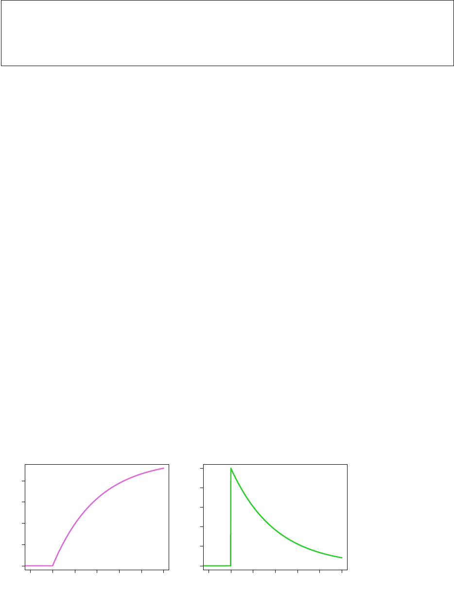
when x ≥ 0 and F (x) = 0 if x < 0. The following provides the CDF (left) and PDF (right) of an exponential
random variable with λ = 0.5:
−1 0 1 2 3 4 5
0.0 0.2 0.4 0.6 0.8
Exponential(0.5)
X
F(x)
−1 0 1 2 3 4 5
0.0 0.1 0.2 0.3 0.4 0.5
Exponential(0.5)
X
p(x)
1-1

1-2 Lecture 1: CDF and EDF
1.2 Statistics and Motivation of Resampling Methods
Given a sample X
1
, ··· , X
n
(not necessarily an IID sample), a statistic S
n
= S(X
1
, ··· , X
n
) is a function of
the sample.
Here are some common examples of a statistic:
• Sample mean (average):
S(X
1
, ··· , X
n
) =
1
n
n
X
i=1
X
i
.
• Sample maximum:
S(X
1
, ··· , X
n
) = max{X
1
, ··· , X
n
}.
• Sample range:
S(X
1
, ··· , X
n
) = max{X
1
, ··· , X
n
} −min{X
1
, ··· , X
n
}.
• Sample variance:
S(X
1
, ··· , X
n
) =
1
n −1
n
X
i=1
X
i
−
¯
X
n
2
,
¯
X
n
=
1
n
n
X
i=1
X
i
.
Here are some useful statistics but might not be so common as the previous few examples:
• Number of observations above a threshold t:
S(X
1
, ··· , X
n
) =
n
X
i=1
I(X
i
> t).
• Rank of the first observation (X
1
):
S(X
1
, ··· , X
n
) = 1 +
n
X
i=2
I(X
i
> X
1
).
If X
1
is the largest number, then S(X
1
, ··· , X
n
) = 1; if X
1
is the smallest number, then S(X
1
, ··· , X
n
) =
n.
• Sample second moment:
S(X
1
, ··· , X
n
) =
1
n
n
X
i=1
X
2
i
.
The sample second moment is a consistent estimator of E(X
2
i
).
Now we assume that our sample X
1
, ··· , X
n
is generated from a sampling distribution. Then the distribution
of these n numbers is determined by the joint CDF F
X
1
,··· ,X
n
(x
1
, ··· , x
n
). In the IID case (or sometimes we
call it a random sample), the joint CDF is the product of the individual CDF’s (and they are all the same
because of being identically distributed). Thus, in the IID case, the individual CDF F (x) = F
X
1
(x) and the
sample size n determines the entire joint CDF.
For a statistic S
n
= S(X
1
, ··· , X
n
), it is a random variable when the sample is random. Because S
n
is a
function of the input data points X
1
, ··· , X
n
, the distribution of S
n
is completely determined by the joint

Lecture 1: CDF and EDF 1-3
CDF of X
1
, ··· , X
n
. Let F
S
n
(x) be the CDF of S
n
. Then F
S
n
(x) is determined by F
X
1
,··· ,X
n
(x
1
, ··· , x
n
),
which under the IID case, is determined by F (x) and n (sample size).
Thus, when X
1
, ··· , X
n
∼ F ,
(F (x), n)
determine
−→ F
X
1
,··· ,X
n
(x
1
, ··· , x
n
)
determine
−→ F
S
n
(x). (1.1)
Mathematically speaking, there is a map Ψ : F × N 7→ F such that
F
S
n
= Ψ(F, n), (1.2)
where F is a collection of all possible CDF’s.
Example. Assume X
1
, ··· , X
n
∼ N (0, 1). Let S
n
=
1
n
P
n
i=1
X
i
be the sample average. Then the CDF
of S
n
is the CDF of N(0, 1/n) by the property of a normal distribution. In this case, F is the CDF of
N(0, 1). Now if we change the sampling distribution from N (0, 1) to N(1, 4), then the sample average S
n
has a CDF of N(1, 4/n). Here you see that the CDF of the sample average, a statistic, changes when the
sampling distribution F changes (and the CDF of S
n
is clearly dependent on the sample size n). This is
what equations (1.1) and (1.2) refer to.
Therefore, a key conclusion is:
Given F and the sample size n, the distribution of any statistic
from the random sample
X
1
, ··· , X
n
is determined.
Even if we cannot analytically write down the function F
S
n
(x), as long as we can sample from F , we can
generate many sets of size-n random samples and compute S
n
of each random sample and find out the
distribution of F
S
n
.
Here you see that the CDF F is very important in analyzing the distribution of any statistic. However, in
practice the CDF F is unknown to us; all we have is the random sample X
1
, ··· , X
n
. So here comes the
question:
Given a random sample X
1
, ··· , X
n
, how can we estimate F ?
1.3 EDF: Empirical Distribution Function
Let first look at the function F (x) more closely. Given a value x
0
,
F (x
0
) = P (X
i
≤ x
0
)
for every i = 1, ··· , n. Namely, F (x
0
) is the probability of the event {X
i
≤ x
0
}.
A natural estimator of a probability of an event is the ratio of such an event in our sample. Thus, we use
b
F
n
(x
0
) =
number of X
i
≤ x
0
total number of observations
=
P
n
i=1
I(X
i
≤ x
0
)
n
=
1
n
n
X
i=1
I(X
i
≤ x
0
) (1.3)
as the estimator of F (x
0
).
For every x
0
, we can use such a quantity as an estimator, so the estimator of the CDF, F (x), is
b
F
n
(x). This
estimator,
b
F
n
(x), is called the empirical distribution function (EDF).
1-4 Lecture 1: CDF and EDF
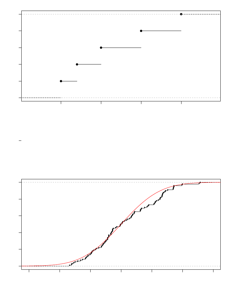
Example. Here is an example of the EDF of 5 observations of 1, 1.2, 1.5, 2, 2.5:
1.0 1.5 2.0 2.5
0.0 0.2 0.4 0.6 0.8 1.0
ecdf(x)
x
Fn(x)
There are 5 jumps, each located at the position of an observation. Moreover, the height of each jump is the
same:
1
5
.
Example. While the previous example might not be look like an idealized CDF, the following provides a
case of EDF versus CDF where we generate n = 100, 1000 random points from the standard normal N(0, 1):
−3 −2 −1 0 1 2 3
0.0 0.2 0.4 0.6 0.8 1.0
n=100
x
Fn(x)
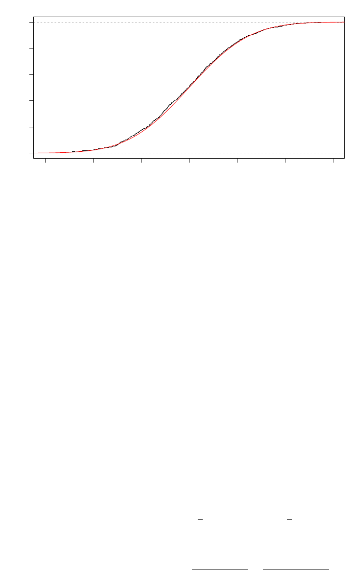
Lecture 1: CDF and EDF 1-5
−3 −2 −1 0 1 2 3
0.0 0.2 0.4 0.6 0.8 1.0
n=1000
x
Fn(x)
The red curve indicates the true CDF of the standard normal. Here you can see that when the sample size
is large, the EDF is pretty close to the true CDF.
1.3.1 Property of EDF
Because EDF is the average of I(X
i
≤ x), we now study the property of I(X
i
≤ x) first. For simplicity, let
Y
i
= I(X
i
≤ x). What is the random variable Y
i
?
Here is the breakdown of Y
i
:
Y
i
=
(
1, if X
i
≤ x
0, if X
i
> x
.
So Y
i
only takes value 0 and 1–so it is actually a Bernoulli random variable! We know that a Bernoulli
random variable has a parameter p that determines the probability of outputing 1. What is the parameter
p for Y
i
?
p = P (Y
i
= 1) = P (X
i
≤ x) = F (x).
Therefore, for a given x,
Y
i
∼ Ber(F (x)).
This implies
E(I(X
i
≤ x)) = E(Y
i
) = F (x)
Var(I(X
i
≤ x)) = Var(Y
i
) = F (x)(1 − F (x))
for a given x.
Now what about
b
F
n
(x)? Recall that
b
F
n
(x) =
1
n
P
n
i=1
I(X
i
≤ x) =
1
n
P
n
i=1
Y
i
. Then
E
b
F
n
(x)
= E(I(X
1
≤ x)) = F (x)
Var
b
F
n
(x)
=
P
n
i=1
Var(Y
i
)
n
2
=
F (x)(1 − F (x))
n
.
What does this tell us about using
b
F
n
(x) as an estimator of F (x)?

1-6 Lecture 1: CDF and EDF
First, at each x,
b
F
n
(x) is an unbiased estimator of F (x):
bias
b
F
n
(x)
= E
b
F
n
(x)
− F (x) = 0.
Second, the variance converges to 0 when n → ∞. By Lemma 0.3, this implies that for a given x,
b
F
n
(x)
P
→ F (x).
i.e.,
b
F
n
(x) is a consistent estimator of F (x).
In addition to the above properties, the EDF also have the following interesting feature: for a given x,
√
n
b
F
n
(x) −F (x)
D
→ N(0, F (x)(1 − F (x))).
Namely,
b
F
n
(x) is asymptotically normally distributed around F (x) with variance F (x)(1 −F (x)).
Example. Assume X
1
, ··· , X
100
∼ F , where F is a uniform distribution over [0, 2]. Questions:
• What will be the expectation of
b
F
n
(0.8)?
−→ E
b
F
n
(0.8)
= F (0.8) = P (x ≤ 0.8) =
Z
0.8
0
1
2
dx = 0.4.
• What will be the variance of
b
F
n
(0.8)?
−→ Var
b
F
n
(0.8)
=
F (0.8)(1 − F (0.8))
100
=
0.4 ×0.6
100
= 2.4 ×10
−3
.
Remark. The above analysis shows that for a given x,
|
b
F
n
(x) −F (x)|
P
→ 0.
This is related to the pointwise convergence in mathematical analysis (you may have learned this in STAT
300). We can extend this result to a uniform sense:
sup
x
|
b
F
n
(x) −F (x)|
P
→ 0.
However, deriving such a uniform convergence requires more involved probability tools so we will not cover
it here. But an important fact is that such a uniform convergence in probability can be established under
some conditions.
Question to think: Think about how to construct a 95% confidence interval of F (x) for a given x.
♦ : The EDF can be used to test if the sample is from a known distribution or two samples are from the
same distribution. The former is called the goodness-of-fit test and the latter is called the two-sample test.
Assume that we want to test if X
1
, ··· , X
n
are from an known distribution F
0
(goodness-of-fit test). There
are three common approaches to carry out this test. The first one is called the KS test (Kolmogorov–Smirnov
test)
1
, where the test statistic is the KS-statistic
T
KS
= sup |
b
F
n
(x) −F
0
(x)|.
1
https://en.wikipedia.org/wiki/Kolmogorov%E2%80%93Smirnov_test

Lecture 1: CDF and EDF 1-7
The second approach is the Cram´er–von Mises test
2
, which uses the Cram´er–von Mises statistic as the test
statistic
T
CM
=
Z
b
F
n
(x) −F
0
(x)
2
dF
0
(x).
The third approach is the Anderson-Darling test
3
and the test statistic is
T
AD
= n
Z
b
F
n
(x) −F
0
(x)
2
F
0
(x)(1 −F
0
(x))
dF
0
(x).
We reject the null hypothesis (H
0
: X
1
, ··· , X
n
∼ F
0
) when the test statistic is greater than some threshold
depending on the significance level α. Note that here we present the test statistics for the goodness-of-fit
test, there are corresponding two-sample test version of each of them.
1.4 Inverse of a CDF
Let X be a continuous random variable with CDF F (x). Let U be a uniform distribution over [0, 1]. Now
we define a new random variable
W = F
−1
(U),
where F
−1
is the inverse of the CDF. What will this random variable W be?
To understand W , we examine its CDF F
W
:
F
W
(w) = P (W ≤ w) = P (F
−1
(U) ≤ w) = P (U ≤ F (w)) =
Z
F (w)
0
1 dx = F (w) − 0 = F (w).
Thus, F
W
(w) = F (w) for every w, which implies that the random variable W has the same CDF as the
random variable X! So this leads a simple way to generate a random variable from F as long as we know
F
−1
. We first generate a random variable U from a uniform distribution over [0, 1]. And then we feed the
generated value into the function F
−1
. The resulting random number, F
−1
(U), has a CDF being F .
This interesting fact also leads to the following result. Consider a random variable V = F (X), where F is
the CDF of X. Then the CDF of V
F
V
(v) = P (V ≤ v) = P (F (X) ≤ v) = P (X ≤ F
−1
(v)) = F (F
−1
(v)) = v
for any v ∈ [0, 1]. Therefore, V is actually a uniform random variable over [0, 1].
Example. Here is a method of generating a random variable X from Exp(λ) from a uniform random variable
over [0, 1]. We have already calculated that for an Exp(λ), the CDF
F (x) = 1 − e
−λx
when x ≥ 0. Thus, F
−1
(u) will be
F
−1
(u) =
−1
λ
log(1 − u).
So the random variable
W = F
−1
(U) =
−1
λ
log(1 − U)
will be an Exp(λ) random variable.
2
https://en.wikipedia.org/wiki/Cram%C3%A9r%E2%80%93von_Mises_criterion
3
https://en.wikipedia.org/wiki/Anderson%E2%80%93Darling_test
