Order Statistics
1 Introduction and Notation
Let X
1
, X
2
, . . . , X
10
be a random sample of size 15 from the uniform distribution over the interval
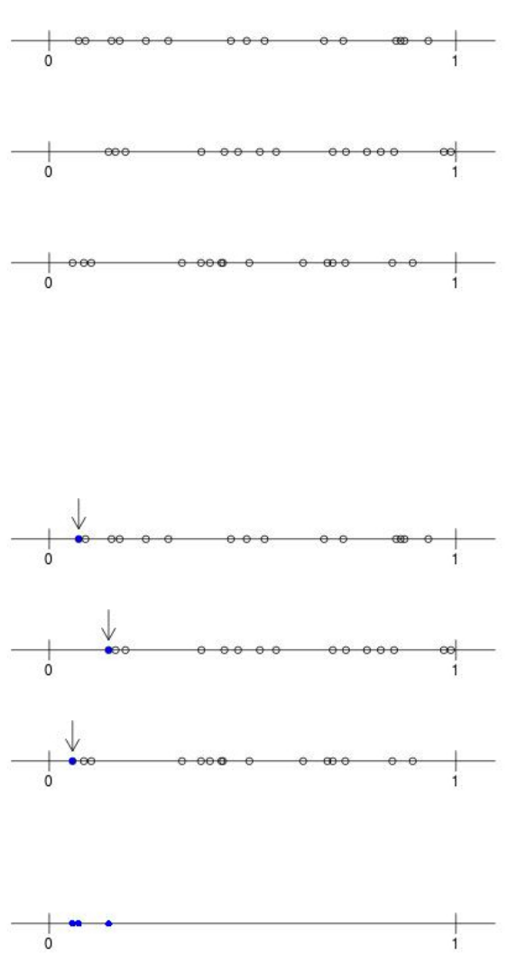
(0, 1). Here are three different realizations realization of such samples.
Because these samples come from a uniform distribution, we expect them to be spread out “ran-
domly” and “evenly” across the interval (0, 1). (You might think that you are seeing some sort of
clustering but keep in mind that you are looking at a measly selection of only three samples. After
collecting more samples I’m sure your view would change!)
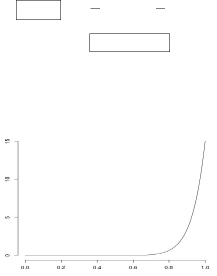
Consider the single smallest value from each of these three samples, highlighted here.
Collect the minimums onto a single graph.
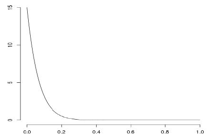
Not surprisingly, they are down towards zero! It would be pretty difficult to get a sample of 15
uniforms on (0, 1) that has a minimum up by the right endpoint of 1. In fact, we will show that if
we kept collecting minimums of samples of size 15, they would have a probability density function
that looks like this.
Notation: Let X
1
, X
2
, . . . , X
n
be a random sample of size n from some distribution. We denote
the order statistics by
X
(1)
= min(X
1
, X
2
, . . . , X
n
)
X
(2)
= the 2nd smallest of X
1
, X
2
, . . . , X
n
.
.
. =
.
.
.
X
(n)
= max(X
1
, X
2
, . . . , X
n
)
(Another commonly used notation is X
1:n
, X
2:n
, . . . , X
n:n
for the min through the max, respec-
tively.)
In what follows, we will derive the distributions and joint distributions for each of these statistics
and groups of these statistics. We will consider continuous random variables only. Imagine
taking a random sample of size 15 from the geometric distribution with some fixed parameter p.
The chances are very high that you will have some repeated values and not see 15 distinct values.
For example, suppose we observe 7 distinct values. While it would make sense to talk about the
minimum or maximum value here, it would not make sense to talk about the 12th largest value in
this case. To further confuse the matter, the next sample might have a different number of distinct
values! Any analysis of the order statistics for this discrete distribution would have to be well-
defined in what would likely be an ad hoc way. (For example, one might define them conditional
on the number of distinct values observed.)
2 The Distribution of the Minimum
Suppose that X
1
, X
2
, . . . , X
n
is a random sample from a continuous distribution with pdf f and
cdf F . We will now derive the pdf for X
(1)
, the minimum value of the sample. For order statistics,
it is usually easier to begin by considering the cdf. The game plan will be to relate the cdf of the
minimum to the behavior of the individual sampled values X
1
, X
2
, . . . , X
n
for which we know the
pdf and cdf.
The cdf for the minimum is
F
X
(1)
(x) = P (X
(1)
≤ x).
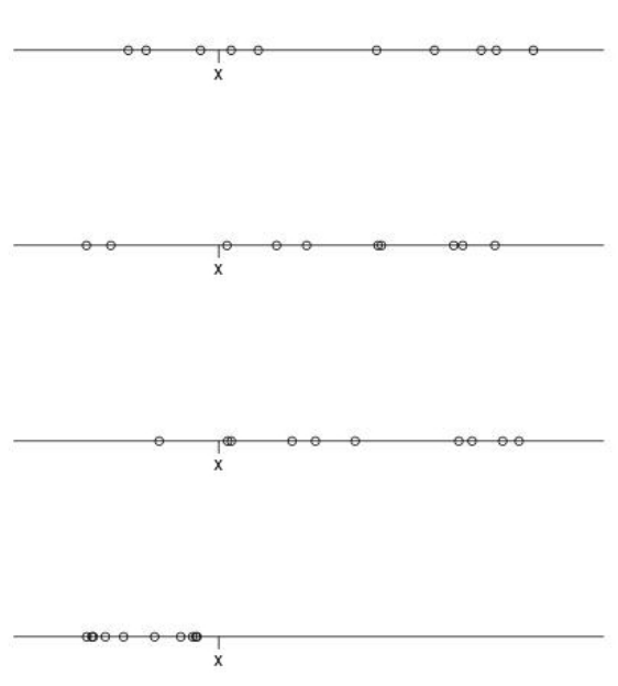
Imagine a random sample falling in such a way that the minimum is below a fixed value x. It might
look like this
or this
or this
or even this.
In other words,
F
X
(1)
(x) = P (X
(1)
≤ x) = P ( at least one of X
1
, X
2
, . . . , X
n
is ≤ x).
There are many ways for the individual X
i
to fall so that the minimum is less than or equal to x.
Considering all of the possibilities is a lot of work! On the other hand, the minimum is greater
than x if and only if all the X
i
are greater than x. So, it is easy to relate the probability P (X
(1)
> x)
back to the individual X
i
. Thus, we consider
F
X
(1)
(x) = P (X
(1)
≤ x) = 1 − P (X
(1)
> x)
= 1 − P ( X
1
> x, X
2
> x, . . . , X
n
> x )
= P (X
1
> x)P (X
2
> x) · · · P (X
n
> x) by independence
= 1 − [P (X
1
> x)]
n
because the X
i
are identically distributed
= 1 − [1 − F (x)]
n
So, we have that the pdf for the minimum is
f
X
(1)
(x) =
d
dx
F
X
(1)
(x) =
d
dx
{1 − [1 − F (x)]
n
}
= n[1 − F (x)]
n−1
f(x)
Going back to the uniform example of Section 1, we had f(x) = I
(0,1)
(x) and
F (x) =
0 , x < 0
x , 0 ≤ x < 1
1 , x ≥ 1.
The pdf for the minimum in this case is
f
X
(1)
(x) = n[1 − x]
n−1
I
(0,∞)
(x).
This is the pdf for the Beta distribution with parameters 1 and n. Thus, we can write
X
(1)
∼ Beta(1, n).
3 The Distribution of the Maximum
Again consider our random sample X
1
, X
2
, . . . , X
n
from a continuous distribution with pdf f and
cdf F . We will now derive the pdf for X
(n)
, the maximum value of the sample. As with the
minimum, we will consider the cdf and try to relate it to the behavior of the individual sampled
values X
1
, X
2
, . . . , X
n
.
The cdf for the minimum is
F
X
(1)
(x) = P (X
(1)
≤ x).
Imagine a random sample falling in such a way that the maximum is below a fixed value x. This
will happen if and only if all of the X
i
are below x.
Thus, we have
F
X
(n)
(x) = P (X
(n)
≤ x)
= P ( X
1
≤ x, X
2
≤ x, . . . , X
n
≤ x )
= P (X
1
≤ x)P (X
2
≤ x) · · · P (X
n
≤ x) by independence
= [P (X
1
≤ x)]
n
because the X
i
are identically distributed
= [F (x)]
n
.
Take the derivative, we get the pdf for the maximum to be
f
X
(n)
(x) =
d
dx
F
X
(1)
(x) =
d
dx
[F (x)]
n
= n[F (x)]
n−1
f(x)
In the case of the random sample of size 15 from the uniform distribution on (0, 1), the pdf is
f
X(n)
(x) = nx
n−1
I
(0,1)
(x)
which is the pdf of the Beta(n, 1) distribution.
Not surprisingly, all most of the probability or “mass” for the maximum is piled up near the right
endpoint of 1.
4 The Joint Distribution of the Minimum and Maximum
Let’s go for the joint cdf of the minimum and the maximum
F
X
(1)
,X
(n)
(x, y) = P (X
(1)
≤ x, X
(n)
≤ y).
It is not clear how to write this in terms of the individual X
i
. Consider instead the relationship
P (X
(n)
≤ y) = P (X
(1)
≤ x, X
(n)
≤ y) + P (X
(1)
> x, X
(n)
≤ y). (1)
We know how to write out the term on the left-hand side. The first term on the right-hand side is
what we want to compute. As for the final term,
P (X
(1)
> x, X
(n)
≤ y),
note that this is zero if x ≥ y. (In this case, P (X
(1)
≤ x, X
(n)
≤ y) = P (X
(n)
≤ y) and (1) gives
us only P (X
(n)
≤ y) = P (X
(n)
≤ y) which is both true and uninteresting! So, we consider the case
that x < y. Note then that
P (X
(1)
> x, X
(n)
≤ y) = P (x < X
1
≤ y, x < X
2
≤ y, . . . , x < X
n
≤ y)
iid
= [P (x < X
1
≤ y)]
n
= [F (y) − F (x)]
n
.

Thus, from (1), we have that
F
X
(1)
,X
(n)
(x, y) = P (X
(1)
≤ x, X
(n)
≤ y)
= P (X
(n)
≤ y) − P (X
(1)
> x, X
(n)
≤ y)
= [F (y)]
n
− [F (y) − F (x)]
n
.
Now the joint pdf is
f
X
(1)
,X
(n)
(x, y) =
d
dx
d
dy
{[F (y)]
n
− [F (y) − F (x)]
n
}
=
d
dx
n[F (y)]
n−1
f(y) − n[F (y) − F (x)]
n−1
f(y)
= n(n − 1)[F (y) − F (x)]
n−2
f(x)f(y).
This hold for x < y and for x and y both in the support of the original distribution.
For the sample of size 15 from the uniform distribution on (0, 1), the joint pdf for the min and max
is
f
X
(1)
,X
(n)
(x, y) = 15 · 14 · [y − x]
13
I
(0,y)
(x) I
(0,1)
(y).
A Heuristic:
Since X
1
, X
2
, . . . , X
n
are assumed to come from a continuous distribution, the min and max are
also continuous and the joint pdf does not represent probability– it is a surface under
which volume represents probability. However, if we bend the rules and think of the joint pdf as
probability, we can develop a heuristic method for remembering it.
Suppose (though it is not true) that
f
X
(1)
,X
(n)
(x, y) = P (X
(1)
= x, X
(n)
= y).
This would mean that we need one value in the sample X
1
, X
2
, . . . , X
n
to fall at x, one value to
fall at y, and the remaining n − 2 values to fall in between.
The “probability” one of the X
i
is x is “like” f(x). (Remember, we are bending the rules here
in order to develop a heuristic. This probability is, of course, actually 0 for a continuous random
variable.)
The “probability” one of the X
i
is y is “like” f(y).
The probability that one of the X
i
is in between x and y is (actually) F (y) − F (x).
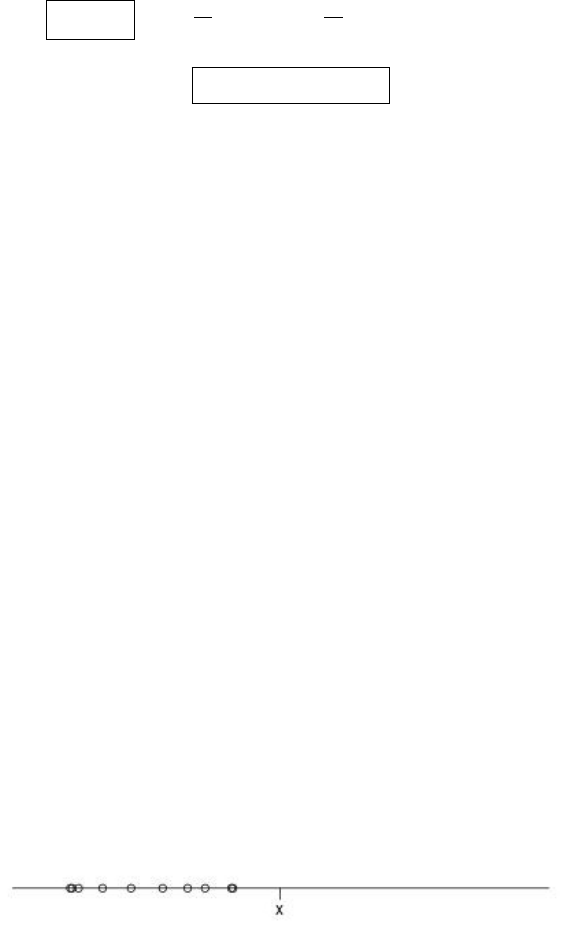
The sample can fall many ways to give us a minimum at x and a maximum at y. For example,
imagine that n = 5. We might get X
3
= x, X
1
= y and the remaining X
2
, X
4
, X
5
in between x and
y.
This would happen with “probability”
f(x)[F (y) − F (x)]
3
f(y).

Another possibility is that we get X
5
= x and X
2
= y and the remaining X
1
, X
3
, X
4
in between x
and y.
This would also happen with “probability”
f(x)[F (y) − F (x)]
3
f(y).
We have to add this “probability” up as many times as there are scenarios. So, let’s count them.
There are 5! different ways to lay down the X
i
. For each one, there are 3! different ways to lay
down the remaining values in between that will result in the same min and max. So, we need to
divide these redundancies out for a total of 5!/3! = (5)(4) ways to get that min at x and max at y.
In general, for a sample of size n, there are n! different ways to lay down the X
i
. For each one,
there are (n − 2)! different ways that result in the same min and max. So, there are a total of
n!/(n − 2)! = n(n − 1) ways to get that
Thus, the “probability” of getting a minimum of x and a maximum of y is
n(n − 1)f(x)[F (y) − F (x)]
n−2
f(y),
which looks an awful lot like the formula we derived above!
5 The Joint Distribution for All of the Order Statistics
We wish now to find the pdf
f
X
(1)
,X
(2)
,...,X
(n)
(x
1
, x
2
, . . . , x
n
).
This time, we will start with the heuristic aid.
Suppose that n = 3 and we want to find
f
X
(1)
,X
(2)
,X
(3)
(x
1
, x
2
, x
3
) “=” P (X
(1)
= x
1
, X
(2)
= x
2
, X
(3)
= x
3
).
The first thing to notice is that this probability will be 0 if we don’t have x
1
< x
2
< x
3
. (Note that
we need strict inequalities here. For a continuous distribution, we will never see repeated values so
the minimum and second smallest, for example, could not take on the same value.)
Fix values x
1
< x
2
< x
3
. How could a sample of size 3 fall so that the minimum is x
1
, the next
smallest is x
2
, and the largest is x
3
? We could observe
X
1
= x
1
, X
2
= x
2
, X
3
= x
3
,
or
X
1
= x
2
, X
2
= x
1
, X
3
= x
3
,
or
X
2
= x
2
, X
2
= x
3
, X
3
= x
1
,
or...
There are 3! possibilities to list. The “probability” for each is f(x
1
)f(x
2
)f(x
3
). Thus,
f
X
(1)
,X
(2)
,X
(3)
(x
1
, x
2
, x
3
) “=” P (X
(1)
= x
1
, X
(2)
= x
2
, X
(3)
= x
3
) = 3!f(x
1
)f(x
2
)f(x
3
).

For general n, we have
f
X
(1)
,X
(2)
,...,X
(n)
(x
1
, x
2
, . . . , x
n
) “=” P (X
(1)
= x
1
, X
(2)
= x
2
, . . . X
(n)
= x
n
)
= n!f(x
1
)f(x
2
) · · · f(x
n
)
which holds for x
1
< x
2
< · · · < x
n
with all x
i
in the support for the original distribution. The
joint pdf is zero otherwise.
The Formalities:
The joint cdf,
P (X
(1)
≤ x
1
, X
(2)
≤ x
2
, . . . , X
(n)
≤ x
n
),
is a little hard to work with. Instead, we consider something similar:
P (y
1
< X
(1)
≤ x
1
, y
2
< X
(2)
≤ x
2
, . . . , y
n
< X
(n)
< x
n
)
for values y
1
< x
1
≤ y
2
< x
2
≤ y
3
< x
3
≤ · · · ≤ y
n
< x
n
.
This can happen if
y
1
< X
1
≤ x
1
, y
2
< X
2
≤ x
2
, . . . , y
n
< X
n
< x
n
,
or if
y
1
< X
5
≤ x
1
, y
2
< X
3
≤ x
2
, . . . , y
n
< X
n−2
< x
n
,
or...
Because of the constraints on the x
i
and y
i
, these are disjoint events. So, we can add these n!
probabilities, which will all be the same, together to get
P (y
1
< X
(1)
≤ x
1
, . . . , y
n
< X
(n)
< x
n
) = n! P (y
1
< X
1
≤ x
1
, . . . , y
n
< X
n
< x
n
).
Note that
P (y
1
< X
1
≤ x
1
, . . . , y
n
< X
n
< x
n
)
indep
=
n
Y
i=1
P (y
i
< X
i
≤ x
i
) =
n
Y
i=1
[F (x
i
) − F (y
i
)].
So,
P (y
1
< X
(1)
≤ x
1
, . . . , y
n
< X
(n)
< x
n
) = n!
n
Y
i=1
[F (x
i
) − F (y
i
)] (2)
The left-hand side is
Z
x
n
y
n
Z
x
n−1
y
n−1
· · ·
Z
x
1
y
1
f
X
(1)
,X
(2)
,...,X
(n)
(u
1
, u
2
, . . . , u
n
) du
1
du
2
. . . , du
n
.
Taking derivatives
d
dx
1
d
dx
2
· · ·
d
dx
n
gives
f
X
(1)
,X
(2)
,...,X
(n)
(x
1
, x
2
, . . . , x
n
)
Differentiating both sides of (2) with respect to x
1
, x
2
, . . . , x
n
gives us
f
X
(1)
,X
(2)
,...,X
(n)
(x
1
, x
2
, . . . , x
n
) = n!f(x
1
)f(x
2
) · · · f(x
n
)
which holds for x
1
< x
2
< · · · , x
n
and all x
i
in the support of the original distribution. The pdf is
zero otherwise.

6 The Distribution of X
(i)
We can get the marginal pdf for the ith order statistic X
(i)
, by taking the joint pdf for all order
statistics from Section 5 and integrating out the unwanted x
j
.
Let’s start by integrating out x
1
. Since the support of the joint pdf for the order statistics includes
the constraint x
1
< x
2
< · · · < x
n
, limits of integration are −∞ to x
2
.
f
X
(2)
,...,X
(n)
(x
2
, . . . , x
n
) =
R
x
2
−∞
f
X
(1)
,X
(2)
,...,X
(n)
(x
1
, x
2
, . . . , x
n
) dx
1
=
R
x
2
−∞
n!f(x
1
)f(x
2
) · · · f(x
n
) dx
1
= n!f(x
2
) · · · f(x
n
)
R
x
2
−∞
f(x
1
) dx
1
= n!f(x
2
) · · · f(x
n
)F (x
2
)
for x
2
< x
3
< · · · < x
n
.
Now let’s integrate out x
2
which goes from −∞ to x
3
.
f
X
(3)
,...,X
(n)
(x
3
, . . . , x
n
) =
R
x
3
−∞
f
X
(2)
,...,X
(n)
(x
2
, . . . , x
n
) dx
2
= n!f(x
3
) · · · f(x
n
)
R
x
3
−∞
F (x
2
)
| {z }
u
f(x
2
) dx
2
| {z }
du
= n!f(x
3
) · · · f(x
n
)
1
2
[F (x
2
)]
2
x
2
=x
3
x
2
=−∞
= n!f(x
3
) · · · f(x
n
)
1
2
([F (x
3
)]
2
− [F (−∞)
| {z }
0
]
2
)
=
n!
2
f(x
3
) · · · f(x
n
)[F (x
3
)]
2
which holds for x
3
< x
4
< · · · < x
n
.
The next time through, we will integrate out x
3
from −∞ to x
4
. Using u = F (x
3
) and du =
f(x
3
) dx
3
, we get
f
X
(4)
,...,X
(n)
(x
4
, . . . , x
n
) =
n!
(3)(2)
f(x
4
) · · · f(x
n
)[F (x
4
)]
3
.
Continue until we reach X
(i)
:
f
X
(i)
,...,X
(n)
(x
i
, . . . , x
n
) =
n!
(i − 1)!
f(x
i
) · · · f(x
n
)[F (x
i
)]
i−1
which holds for x
i
< x
i+1
< · · · < x
n
.
Now, we start integrating off x’s from the other side.
f
X
(i)
,...,X
(n−1)
(x
i
, . . . , x
n−1
) =
R
∞
x
n−1
f
X
(i)
,...,X
(n−1)
(x
i
, . . . , x
n
) dx
n
=
n!
(i−1)!
f(x
i
) · · · f(x
n−1
)[F (x
i
)]
i−1
R
∞
x
n−1
f(x
n
) dx
n
=
n!
(i−1)!
f(x
i
) · · · f(x
n−1
)[F (x
i
)]
i−1
[1 − F (x
n−1
)]

for x
i
< x
i+1
< · · · , x
n−1
.
f
X
(i)
,...,X
(n−2)
(x
i
, . . . , x
n−2
) =
R
∞
x
n−2
f
X
(i)
,...,X
(n−1)
(x
i
, . . . , x
n−1
) dx
n−1
=
n!
(i−1)!
f(x
i
) · · · f(x
n−2
)[F (x
i
)]
i−1
R
∞
x
n−2
f(x
n−1
)[1 − F (x
n−1
)] dx
n−1
Letting u = 1 − F (x
n−1
) and du = −f(x
n−1
) dx
n−1
, we get
f
X
(i)
,...,X
(n−2)
(x
i
, . . . , x
n−2
) =
n!
(i−1)!
f(x
i
) · · · f(x
n−2
)[F (x
i
)]
i−1
n
−
1
2
[1 − F (x
n−1
)]
2
o
x
n−1
=∞
x
n−1
=x
n−2
=
n!
2(i−1)!
f(x
i
) · · · f(x
n−2
)[F (x
i
)]
i−1
[1 − F (x
n−2
)]
2
for x
i
< x
i+1
, · · · < x
n−2
.
The next time through we will integrate out x
n−2
from x
n−3
to ∞. Note that
R
∞
x
n−3
f(x
n−2
)[1 − F (x
n−2
)
| {z }
u
]
2
dx
n−2
= −
1
3
[1 − F (x
n−2
)]
3
x
n−2
=∞
x
n−2
=x
n−3
=
1
3
[1 − F (x
n−3
)]
3
.
Thus,
f
X
(i)
,...,X
(n−3)
(x
i
, . . . , x
n−3
) =
n!
(3)(2)(i − 1)!
f(x
i
) · · · f(x
n−3
)[F (x
i
)]
i−1
[1 − F (x
n−3
)]
3
for x
i
< x
i+1
< · · · < x
n−3
.
Continuing all the way down to the marginal pdf for X
(i)
alone, we get
f
X
(i)
=
n!
(n−i)!(i−1)!
[F (x
i
)]
i−1
f(x
i
)[1 − F (x
n−3
)]
n−i
for −∞ < x
i
< ∞. (← This may be further restricted by indicators in f(x
i
).)
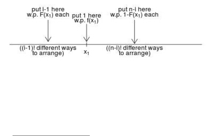
The Heuristic:
We once again will think of the continuous random variables X
1
, X
2
, . . . , X
n
as discrete and f
X
(i)
(x
i
)
as the “probability” that the ith order statistic is at x
i
. First not that there are n! different ways to
arrange the x
0
s. We need to put 1 at x
i
, which will happen with “probability” f(x
i
). We need to
put i − 1 below x
i
, which will happen with probability [F (x
i
)]
i−1
and we need to put n− i above x
i
,
which will happen with probability [1 − F (x
i
)]
n−i
. There are (i − 1)! different ways to arrange the
x’s chosen to go below x
i
. These arrangements are redundant and need to be divided out. Hence,
we have (i − 1)! in the denominator. There are (n − i)! different ways to arrange the x’s chosen to
go above x
i
. These arrangements are also redundant and need to be divided out. Thus, we also
have (n − i)! in the denominator.
7 The Joint Distribution of X
(i)
and X
(j)
for i < j
As in Section 6, one could start with the joint pdf for all of the order statistics and integrate out
the unwanted ones. The result will be
f
X
(i)
,X
(j)
(x
i
, x
j
) =
n!
(i − 1)!(j − i − 1)!(n − j)!
[F (x
i
)]
i−1
f(x
i
)[F (x
j
)−F (x
i
)]
j−i−1
f(x
j
)[1−F (x
j
)]
n−j
for −∞ < x
i
< x
j
< ∞.
Can you convince yourself of this heuristically?
